Analysis of Cohort Studies

Cohort studies are observational studies. We analyze cohort studies using tabular methods and ML methods.

Tabular methods

You can use a 2x2 table to calculate a bunch of stuff.

	O+	O-
E+	a	b
E-	c	d

Risk Ratio is the probability of the outcome in the exposed divided by the probability of outcome in unexposed group:

$$RR = \frac{\frac{a}{a+c}}{\frac{b}{b+d}}$$ $$OR = \frac{a/c}{b/d}$$

You really use CIs If the CI includes one, it is not significant. Now for continuous distributions, you use a t-test. Note that you can’t use the z-test because with that you are assuming that you know the population variance!

Linear Regression

Note that $y = \Beta_0 + \Beta_1X$ will give you an average.

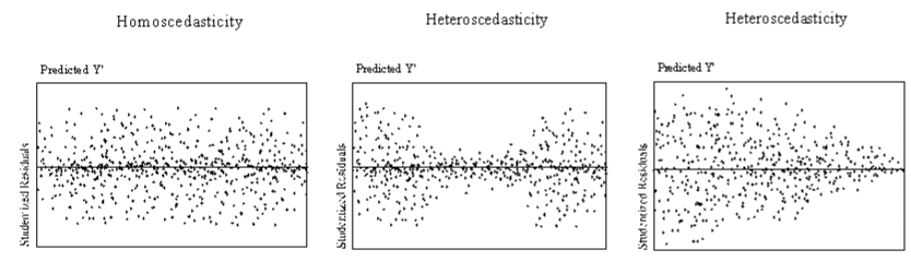
Error terms: assume normality, assume constant variance (homoscedasticity, hetero otherwise).

Use in Hypothesis Testing for Cohort Studies

You make a table, get the regression equation, you are now trying to make epidemiological assertions.

You can calculate the t-statistic. Another way is

Non-parametric bootstrap methods: Sample randomly (with replacement), run regression for each get $\Beta_n$ for $n$ runs. Sort by values, get 2.5th and 97.5th percentiles, compare with… TODO?

If you approach with a causal lens, you can answer a lot of epi questions. DAGs are good for this (Rothman calls them SWIGs, Single World Intervention Graphs). You express a relationship and estimate its effect size with regression (just one way, there are others) and DAGs. You can draw these things:

A Main Effect is simply X -> Y.

Covariates affect outcomes but are not associated with other features. X -> Y and confounder C -> Y.

Confounders are outside the causal pathway that distort the causal relationship between effect and outcome. Now you can test if something is a confounder by having

$$\begin{align*} y &= \Beta_0 + \Beta_1X \text{ as crude model} \\ y &= \Beta_0 + \Beta_1X +\Beta_2C \text{ as adjusted model} \end{align*}$$

Now if $\Beta_1$ changes across these two by more than $\plusmn10\%$, you conclude that $C$ is a confounder.

Statistical Interaction is another. X -> C -> Y in addition to X -> Y.

$$\begin{align*} y &= \Beta_0 + \Beta_1X \text{ as crude model} \\ y &= \Beta_0 + \Beta_1X +\Beta_2C +\Beta_3X*C \text{ as adjusted model} \end{align*}$$

Now you look at $\Beta_3$. If it is more than zero you conclude that there is some interactions.

Another is Mediation: X -> M -> Y

$$\begin{align*} Y &= \Beta_0 + \Beta_1X \\ M &= \Beta_0 + \Beta_1X \\ Y &= \Beta_0 + \Beta_1M \\ Y &= \Beta_0 + \Beta_{1X}X +\Beta_2M \end{align*}$$

Now: if any $\Beta_1$ in any one of models 1-3 is low, you conclude there is very little mediation.

note

Cohort studies, DAGs, and regression work as a unified framework for Computational Epidemiology.

TODO

• Why must the outcome be continuous if the exposure is binary for a regression?